Introduction to Principal Component Analysis – Part 2

Introduction:-

As we say

“Too much of anything is good for nothing!“

Imagine this – you are working on a large scale data science project. What happens when the given data set has too many variables? Here are few possible situations which you might come across:

Imagine you’re working on large scale Data Science project. What happens when the given dataset has too many variables. I’m listing out couple of possible situation that you might come across-

1. You may find a large group of variables is redundant.
2. You may find that most of the variables are correlated.
3. You might lose patience and you may run your model on the whole data . And as popular notion goes in Machine Learning,” Garbage in , Garbage out” . So this may return poor accuracy .
4. You might become indecisive about your next step.
5. You’d want to find out a strategy to find out few important variables from your dataset.

Trust me, dealing with such situations isn’t as difficult as it sounds. Statistical techniques such as factor analysis and principal component analysis , Singular Value Decomposition help to overcome such difficulties.

What is PCA:-

PCA is a linear transformation method. In PCA, we are interested to find the directions (components) that maximize the variance in our dataset

In simple words, via PCA, we are projecting the entire set of data (without class labels) onto a different subspace & we try to determine a suitable subspace to distinguish between patterns that belong to different classes. In layman ,let’s say PCA tries to find the axes with maximum variances where the data is most spread (within a class, since PCA treats the whole data set as one class).

So the Principal component analysis enables us to create and use a reduced set of variables, which are called principal factors or Principal Components. A reduced set is much easier to analyze and interpret. To study a data set that results in the estimation of roughly 500 parameters may be difficult, but if we could reduce these to 5 it would certainly make our day. In the following post you’ll see how to achieve substantial dimension reduction.

But what is a “good” subspace?:-

Let’s assume that our goal is to reduce the dimensions of a n-dimensional dataset by projecting it onto a k-dimensional subspace (where k<n). So, how do we know what size we should choose for k, and how do we know if we have a feature space that represents our data “well”?

We compute eigenvectors (the components) from our data set (or alternatively calculate them from the covariance matrix). Each of those eigenvectors is associated with an eigenvalue, which tell us about the “length” or “magnitude” of the eigenvectors. If we observe that all the eigenvalues are of very similar magnitude, this is a good indicator that our data is already in a “good” subspace. Or if some of the eigenvalues are much higher than others, we might be interested in keeping only those eigenvectors with the much larger eigenvalues, since they contain more information about our data distribution. Vice versa, eigenvalues that are close to 0 are less informative and we might consider in dropping those when we construct the new feature subspace.

Summarizing the PCA approach:-

Let’s summarize the approach that we’d be taking in this following post-

1. Take the whole n dimensional dataset ignoring the class labels
2. Normalize/ Standardize the data
3. Compute Covariance matrix of the whole dataset.
4. Compute the Eigenvectors & their corresponding Eigenvalues
5. Sort the Eigenvectors by decreasing Eigenvalues and choose k Eigenvectors with the largest Eigenvalues from n*k dimensional matrix W (where every column represents an Eigenvector)
6. Use this n*k  Eigenvector matrix to transform the samples on to new subspace. Use the principal components to transform the data – Reduce the dimensionality of the data. This can be summarized by the mathematical equation:  Y=W T *X (where X is a n*1 dimensional vector representing one sample, and Y is the transformed k*1 dimensional vector representing one sample)

Step 4 to 6 could be new to you but trust me, though this way may seem a little out of the blue but it’s worth it. The mystic here is to find the eigenvectors and eigenvalues of the covariance matrix of a dataset. I don’t want to delve deep into the maths behind calculating the covariance matrix as well as finding the eigenvectors and eigenvalues of the covariance matrix and why the eigenvalues and eigenvectors of the covariance matrix turn out to be the principal components of a dataset but just want to give a swift overview. For a mathematical proof on why the eigenvalues and eigenvectors of the covariance matrix turn out to be the principal components of a dataset, I refer the interested reader to the chapter about PCA of Marsland, S. (2015) pp.134. For persons who want to understand the maths behind eigenvectors and eigenvalues, I recommend to look these terms up into text books about linear algebra. But now, step by step (this example is based on Smith, L.I. (2002)):

Step1. Generate Data:-

The problem of multi-dimensional data is its visualization, which would make it quite tough to follow our example principal component analysis (at least visually). We could also choose a 3-dimensional sample data set for the following examples but that would make little tough to understand the visualization of datapoints ( In my next post I’ll extrapolate this PCA approach on more than 3 dimensional dataset  ),And since the goal of the PCA in an “Dimensionality Reduction” application is to drop at least one of the dimensions, I find it more intuitive and visually appealing to start with a 2-dimensional dataset that we reduce to an 1-dimensional dataset by dropping 1 dimension.

PCA behavior is easiest to visualize by looking at a two-dimensional dataset. Consider the following 350 data points:

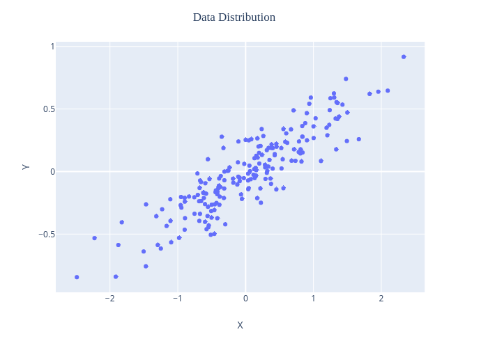
We can clearly see that  it is clear that there is a nearly linear relationship between the x and y variables. 

But the problem setting here is slightly different: rather than attempting to predict the y values from the x values, the unsupervised learning problem attempts to learn about the relationship between the x and y values.

In principal component analysis, this relationship is quantified by finding a list of the principal axes in the data, and using those axes to describe the dataset

Step2:- Standardize the data:-

The principal components are supplied with normalized version of original predictors. This is because, the original predictors may have different scales. For example: Imagine a data set with variables’ measuring units as gallons, kilometers, light years etc. It is definite that the scale of variances in these variables will be large.

Performing PCA on un-normalized variables will lead to insanely large loadings for variables with high variance. In turn, this will lead to dependence of a principal component on the variable with high variance. This is undesirable.

So next, standardize the X matrix so that each column mean is 0 and each column variance is 1. Call this matrix Z or X_std. Each column is a vector variable, zi,i=1,…,p. The main idea behind principal component analysis is to derive a linear function y for each of the vector variables zi. This linear function possesses an extremely important property; namely, its variance is maximized.

Step 3. Compute Covariance Matrix

Variance : It is a measure of the variability or it simply measures how spread the data set is. Mathematically, it is the average squared deviation from the mean score. We use the following formula to compute variance var(x).

Step 3. Compute Covariance Matrix

Co-variance: It is a measure of the extent to which corresponding elements from two sets of ordered data move in the same direction. Formula is shown below denoted by cov(x,y) as the co-variance of x and y.

Here, xi is the value of x in ith dimension.x bar and y bar denote the corresponding mean values.One way to observe the covariance is how interrelated two data sets are.

What are Principal Components ?:-

Before we compute PCs ,Eigenvectors and Eigenvalues , Let’s understand about them a little.

 Principal components:- A principal component is a normalized linear combination of the original predictors in a data set. Let’s say we have a set of predictors as X1, X2,…, Xp . AS we know that Principal components analysis (PCA) produces a low-dimensional representation of a data set.  And how it does that is – It finds a sequence of linear combinations of the variables that have maximal variance and are mutually uncorrelated and these uncorrelated linear combination of variables become Principal components of your data.

This transformation is defined in such a way that the first principal component has the largest possible variance (that is, accounts for as much of the variability in the data as possible), and each succeeding component in turn has the highest variance possible under the constraint that it is orthogonal to the preceding components. The resulting vectors (each being a linear combination of the variables and containing n observations) are an uncorrelated orthogonal basis set.

Kindly note that the first principal component has the largest variance followed by the second principal component and so on & the variance in principal components decreases from the first principal component to the last one.

First principal component (z1) :-

The first principal component of a set of features X1, X2,…, Xp is the normalized linear combination of the features

Z1=ϕ11X1+ϕ21X2+ϕ31X2+…+ϕp1Xp

with the largest variance. By normalized, we mean that ∑j=1pϕj12=1; the elements ϕ11,…, ϕp1 are the loadings of the first principal component; together, the loadings make up the principal component loading vector, ϕ1 = (ϕ11, ϕ21, … ϕp1)T.

The loadings are constrained so that the sum of their squares is equal to one; otherwise, setting these elements to be arbitrarily large in absolute value could result in an arbitrarily large variance

Second principal component ( Z2):- It is also a linear combination of original predictors which captures the remaining variance in the data set and is uncorrelated with  Z1. In other words, the correlation between first and second component should be zero. It can be represented as:

Z2=ϕ12X1+ϕ22X2+ϕ32X2+…+ϕp2Xp

Step 4. Compute the Eigenvectors & their corresponding Eigenvalues

Eigenvectors & Eigen Value & Eigen pairs:-

Eigenvectors represent directions. Think of plotting your data on a multidimensional scatterplot. Then one can think of an individual eigenvector as a particular “direction” in your scatterplot of data. Eigenvalues represent magnitude, or importance. Bigger eigenvalues correlate with more important directions.

Finally, we make an assumption that more variability in a particular direction correlates with explaining the behavior of the dependent variable. Lots of variability usually indicates signal, whereas little variability usually indicates noise. Thus, the more variability there is in a particular direction is, theoretically, indicative of something important we want to detect.

Thus, PCA is a method that brings together:

1. A measure of how each variable is associated with one another. (Covariance matrix.)
2. The directions in which our data are dispersed (Eigenvectors).
3. The relative importance of these different directions (Eigenvalues).

PCA combines our predictors and allows us to drop the eigenvectors that are relatively unimportant.

Step 5. Sort the Eigenvectors by decreasing Eigenvalues and choose k Eigenvectors with the largest Eigenvalues from n*k dimensional matrix W

If the two components are uncorrelated, their directions should be orthogonal (image below). This image is based on a simulated data with 2 predictors. Notice the direction of the components, as expected they are orthogonal. This suggests the correlation b/w these components in zero.

These vectors represent the principal axes of the data, and the length of the vector is an indication of how “important” that axis is in describing the distribution of the data—more precisely, it is a measure of the variance of the data when projected onto that axis. The projection of each data point onto the principal axes are the “principal components” of the data.

So by now we’ve understood using PCA for dimensionality reduction involves zeroing out one or more of the smallest principal components, resulting in a lower-dimensional projection of the data that preserves the maximal data variance.

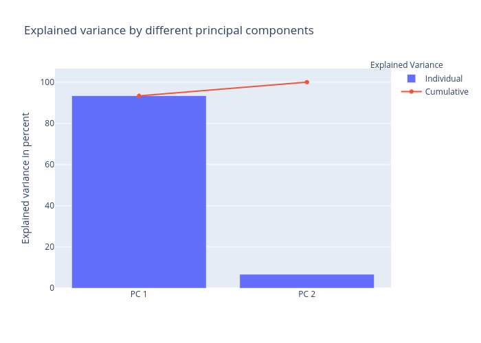
Once we have found the Eigenvectors and eigenvalues of a dataset we can finally use these vectors (which are the principal components of the dataset) to reduce the dimensionality of the data, that is to project the data onto the principal components. As we can see contribution by first Principal Component entails to  ~94% of the total variation  & contribution by 2nd principal component is so less i.e. ~6% that we can easily drop it.

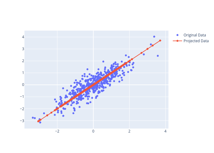
Step 6. Projection Onto the New Feature Space

The light points are the original data, while the dark points are the projected version. This makes clear what a PCA dimensionality reduction means: the information along the least important principal axis or axes is removed, leaving only the component(s) of the data with the highest variance. The fraction of variance that is cut out (proportional to the spread of points about the line formed in this figure) is roughly a measure of how much “information” is discarded in this reduction of dimensionality.

This reduced-dimension dataset is in some senses “good enough” to encode the most important relationships between the points: despite reducing the dimension of the data by 50%, the overall relationship between the data points are mostly preserved.