
Introduction
In this article, we’ll talk about what is Word2Vec Model ,different types of it. Then we’ll understand SkipGram Model architecture in more detail.
“You should know a word by the company it keeps.”
The Word2Vec technique is based on a feed-forward, fully connected architecture. To give an overview of word2vec algorithm ,let’s train a neural network to do the following. Given a specific word in the middle of a sentence (the input word), look at the words nearby and pick one at random. The network is going to tell us the probability for every word in our vocabulary of being the “nearby word” that we chose. When I say “nearby”, there is actually a “window size” parameter to the algorithm. A typical window size might be 5, meaning 5 words behind and 5 words ahead (10 in total). The output probabilities are going to relate to how likely it is find each vocabulary word nearby our input word.
For example, if you gave the trained network the input word “San”, the output probabilities are going to be much higher for words like “Diego” and “Francisco” than for unrelated words like “Apple” and “Orange”.
We’ll train the neural network to do this by feeding it word pairs found in our training documents. The below example shows some of the training samples (word pairs) we would take from the sentence “PM Modi and the American president Trump addressed the Houston rally.” I’ve used a small window size of 2 just for the example. The word highlighted in orange is the input word.
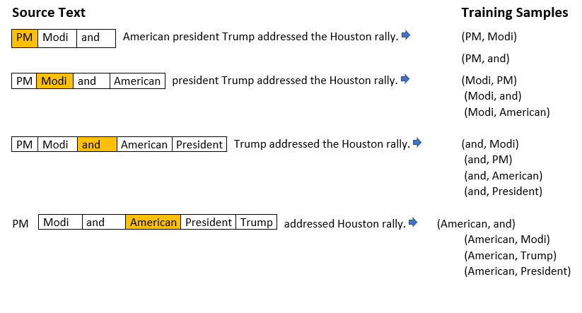
The network is going to learn the statistics from the number of times each pairing shows up. So, for example, the network is probably going to get many more training samples of (“San”, “Diego”) & (“San” , “Francisco”) than it is of (“San”, “York”). When the training is finished, if you give it the word “San” as input, then it will output a much higher probability for “Diego” or “Francisco” than it will for “York”.
In our example above the network is probably going to get many more training samples of (“PM”, “Modi”) than it is of (“PM”, “Trump”). When the training is finished, if you give it the word “Modi” as input, then it will output a much higher probability for “PM” than it will for “president” or “Trump“.
During training, word2vec actually picks a random window size between 1 and window_size. This has the (indirect) effect of giving different weight to the context words based on their distance from the center word. We’ll discuss this further.
Different types in Word2vec
Word2vec comes in two variants–the skip-gram model and the Continuous Bag-of-Words (CBOW) model-
- Skip-grams (SG): Predict context words (position independent) given center word.
- Continuous Bag of Words (CBOW): Predict center word from (bag of) context word.
Skip-gram Model Architecture
First of all, you know you can’t feed a word just as a text string to a neural network, so we need a way to represent the words to the network. To do this, we first build a vocabulary of words from our training documents–let’s say we have a vocabulary of 10,000 unique words. We’re going to represent an input word like “ants” as a one-hot vector. This vector will have 10,000 components (one for every word in our vocabulary) and we’ll place a “1” in the position corresponding to the word “ants”, and 0s in all of the other positions. The output of the network is a single vector (also with 10,000 components) containing, for every word in our vocabulary, the probability that a randomly selected nearby word is that vocabulary word. Here’s the architecture of our neural network.
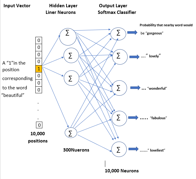 Fig: SkipGram Model Architecture
There is no activation function on the hidden layer neurons, but the output neurons use softmax. Kindly note that when training this network on word pairs, the input is a one-hot vector representing the input word and the training output is also a one-hot vector representing the output word. But when you evaluate the trained network on an input word, the output vector will actually be a probability distribution (i.e., a bunch of floating point values, not a one-hot vector).
The Hidden Layer
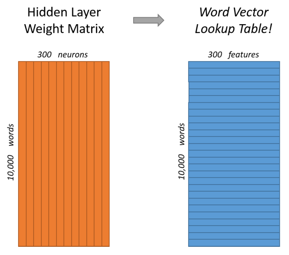
For our example, we’re going to say that we’re learning word vectors with 300 features. So the hidden layer is going to be represented by a weight matrix with 10,000 rows (one for every word in our vocabulary) and 300 columns (one for every hidden neuron).
300 features is what Google used in their published model trained on the Google news dataset (you can download it from here). The number of features is a “hyper parameter” (which is nothing but the Embedding Dimension of each word) that you would just have to tune to your application (that is, try different values and see what yields the best results).
General approach for dealing with words in your text data is to one-hot encode your text. You will have thousands or millions of unique words in your text vocabulary. Computations with such one-hot encoded vectors for these words will be very inefficient because most values in your one-hot vector will be 0. So, the matrix calculation that will happen in between a one-hot vector and a first hidden layer will result in a output that will have mostly 0 values .
We use embeddings to solve this problem and greatly improve the efficiency of our network.Embeddings are just like a fully-connected layer. We will call this layer as—embedding layer and the weights as — embedding weights.
Now, instead of doing the matrix multiplication between the inputs and hidden layer we directly grab the values from embedding weight matrix. We can do this because the multiplication of one-hot vector with weight matrix returns the row of the matrix corresponding to the index of ‘1’ input unit .If you look at the rows of this weight matrix, these are actually what will be our word vectors.
If you multiply a 1 x 10,000 one-hot vector by a 10,000 x 300 matrix, it will effectively just select the matrix row corresponding to the “1”. Here’s a small example to give you a visual.
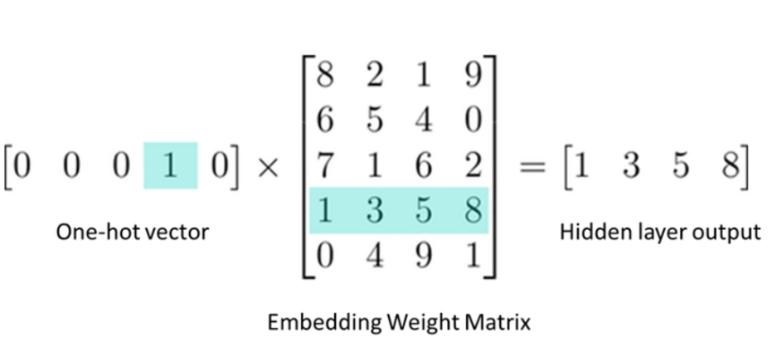
So, we use this Weight Matrix as lookup table. We encode the words as integers, for example ‘cool’ is encoded as 512, ‘hot’ is encoded as 764. Then to get hidden layer output value for ‘cool’ we just simply need to lookup the 512th row in the weight matrix. This process is called Embedding Lookup. The number of dimension in the hidden layer output is the embedding dimension.
Kindly note that at the very beginning of training, all weights in the Embedding matrix are initialized to random values.
Note: – Quality of word embedding increases with higher dimensionality. However, after reaching some threshold, the marginal gain will diminish. Typically, the dimensionality of the vectors is set to be between 100 and 1,000.
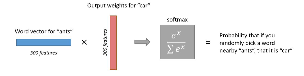
Output Layer
The 1 x 300 word vector for “ants” then gets fed to the output layer. In order to guarantee a probability based representation of the output word, a softmax activation function is used in the output layer and the following error function E is adopted during training:
![]()
![]()
Kindly note that at the very beginning of training, all weights in the Output Matrix are set to 0.
Challenges
You may have noticed that the skip-gram neural network contains a huge number of weights… For our example with 300 features and a vocab of 10,000 words, that’s 3M weights in the hidden layer and output layer each. Training this on a large dataset would be prohibitive, so the word2vec authors introduced a number of tweaks to make training feasible.
We’ll cover this in our next post. So stay tuned!!
Article Credit:-
Name: Praveen Kumar Anwla
Founder: TowardsMachineLearning.Org Linkedin


