Introduction:-

In the article “OpenCV: Beginning for the Computer Vision enthusiast”, we’ll focus on What and why we use OpenCV for Computer Vision, Reading, writing and displaying the images, Color spaces in OpenCV, Resizing, Rotation, translation of the images, Thresholding in OpenCV, different Image enhancement techniques.

Computer vision is one of the hottest and the trending field now-a-days, it is gaining the momentum in terms of Research, Real time application and the industrial usage. The computer vision applications are being used in each type of industry whether it is medical or the automobiles or any other. We can observe some of the examples like the computer vision enabled cameras mounted on the Roads identifying whether a person is wearing the helmet or not, identifying the license plate no.  to identify the particular vehicle, in medical areas we use the computer vision model for  biomedical image segmentation, we are classifying the diseases based on the X-ray, Plant diseases identification, autonomous self-driving, Face detection-based security system, autonomous Drone and there are far many more applications, and these are expanding very rapidly.

Researchers are working on making the algorithms faster, accurate and computer efficient, and the industry is looking for developers in order to put the algorithms in their use.

So, as the computer vision applications are expanding in the industries, Peoples are getting attracted towards its and searching for the various recourses to learn, so in this article we are going the cover the OpenCV library that will help you to start your computer vision journey.

OpenCV is the most popular CV library around, it has thousands of functions that’s helps us in the image processing tasks, but often beginner find it little tough to navigate as there are many functions. It can become daunting to understand the wide variety of functions available, Gauge which function to use for your particular problem.

So, in this article we are going to cover the basic and the most used function in the OpenCV with the detailed explanation along with the implementation in python, this article will help the beginner to dive into the ocean of the computer vision.

 Table of content-

• What and why we use OpenCV for computer vision?
• Reading, writing and displaying the images
• Color spaces in OpenCV
• Resizing, Rotation, translation of the images
• Thresholding in OpenCV
• Image enhancement

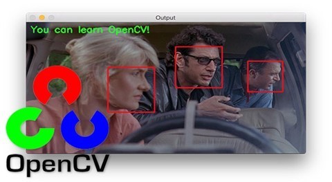
What and why we use OpenCV for computer vision?

OpenCV is an open-source computer vision library, it is referred as the base for the computer vision enthusiast, OpenCV has handful of function which is very much useful in building the computer vision projects. OpenCV was designed for computational efficiency and with a strong focus on real-time applications. It is written in C/C++ so it is fast and efficient. It’s mainly used in image processing, video processing, object detection etc. The library has interfaces for multiple languages, including Python, Java, and C++. It has been severing the developers in computer vision field for a very long time.

Now, we will be learning about some functions that make the task of developing and understanding computer vision models easier to you.

Reading, writing and displaying the images:-

Human being has a capability to see the image and understand the visuals but, have you ever wondered how a computer sees the same image?

I am sure many of you have had that though. So, the obvious answer is the array of pixels.

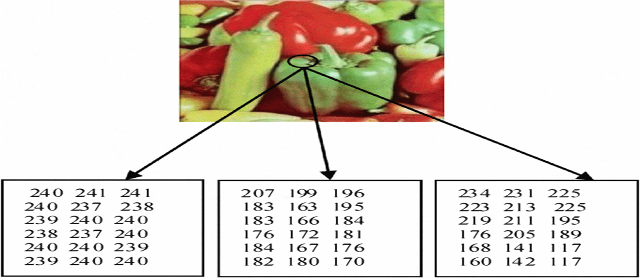
Above fig. shows arrays of pixels corresponding to the RGB image, the three arrays are for the 3 channels of an RGB image i.e. Red, Green, and Blue.

In OpenCV we have a imread() function, which basically reads the images, Imshow() function to output the image and  imwrite() function to save the image in directory.

By default, the imread function reads images in the BGR format. We can read images in different formats using extra flags in the imread function.

• IMREAD_COLOR : Default flag for loading  the image.
• IMREAD_GRAYSCALE : Flag to load the image in grayscale mode.
• IMREAD_UNCHANGED : It specifies to load an image as such including  alpha channel( alpha channel stores the transparency information).

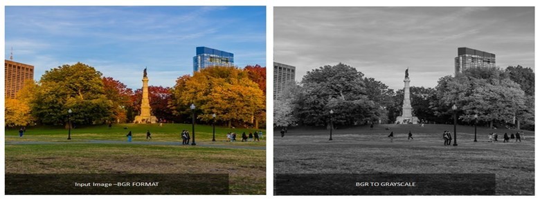
Color spaces in OpenCV:-

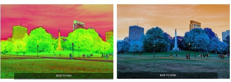
Whenever we are working with the images we need image in different-different format such as RGB, Grayscale, HSV, LAB. OpenCV provides us a handful function cvtColor() for the conversion of the image in different-different format.

We need to give at least two parameters to function; the Input image and color code.​

• BGR TO GRAY  :  cvtColor(input image,COLOR_BGR2GRAY)​
• BGR TO RGB    :  cvtColor( input image,COLOR_BGR2RGB)​
• BGR TO HSV    :  cvtColor(img,COLOR_BGR2HSV)​
• BGR TO LAB     :  cvtColor(img,COLOR_BGR2LAB)​

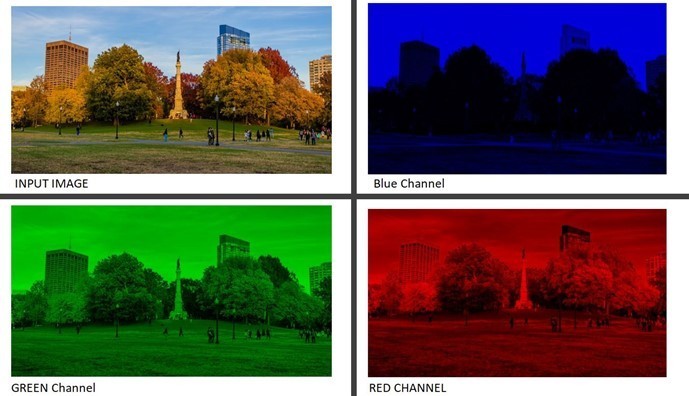
Apart from different color spaces conversion we can also split the image in their respective channels, An RGB image has 3 channels while the gray scale has only one channel. For this we basically uses two function  split() + merge()

The split function will split the R,G,B matrix then using the merge function we can merge R or G or B matrix with zero matrix.

• • For Blue Channel     : merge([B,0,0])
  • For Green Channel   : merge([0,G,0])
  • For Red Channel      : merge([0,0,R])

Resizing, Rotation & Translation :-

Resizing, Rotation, Translation all these are the basic steps we perform, during the image processing for any project. OpenCV has functions for all of these operations.

Let’s have a look on them one by one.

Resizing –

Computer vision model works with fixed size input, In many cases while we builds a model, we don’t have the same size of images, so we have to resize them to feed into the network. Apart of this sometimes we have a fixed size inputs but we need to reduce to the particular size in order to reduce the computational cost So, Here the openCV’s resize function comes in play.

OpenCV has Different interpolation and down sampling methods, which can be used:

1. INTER_NEAREST :  Nearest neighbor interpolation, This is fast but no that efficient.
2. INTER_LINEAR :  Bilinear interpolation, used when zooming is required
3. INTER_AREA :  Resampling using pixel area relation, used to shrink the image
4. INTER_CUBIC :  Bicubic interpolation over 4×4 pixel neighborhood, used when       zooming the image, more computationally expensive but better result than the linear interpolation.
5. INTER_LANCZOS4 : Lanczos interpolation over 8×8 neighborhood, not used generally.

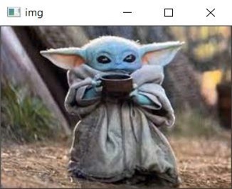
                        Image: Input Image

Rotation & Translation-

Suppose we want to train a model, but not have sufficient no. images, then data argumentation comes in play to fulfill the need of data hungry model. Rotation and translation both are the basic image argumentation techniques.

Rotation

As the name suggests, it involves rotating the image at an arbitrary. Rotating an image in the OpenCV required two functions first is getRotationMatrix2D which gives you Rotation matrix and second is wrapAffine function.

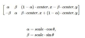
Implementation in python is shown below-

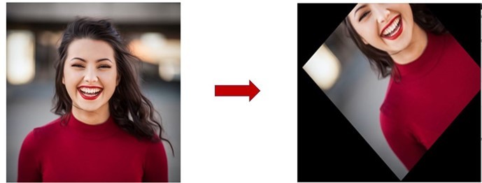
Image translation

It is a geometric transformation that maps the position of every object in the image to a new location in the final output image. After the translation operation, an object present at location (x,y) in the input image is shifted to a new position (X,Y):

X = x + dx

Y = y + dy

Here, dx and dy are the respective translations along different dimensions.

Similar to rotation it also required two thing translation matrix(we have to hardcode it) and the wrapAffine function.

Thresholding in OpenCV:-

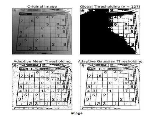
Thresholding is a very popular segmentation technique, used for image partitioning into a foreground and background. Thresholding is a technique of assignment of pixel values in relation to the threshold value provided, if the pixel value is less than the threshold then it is set to 0(min) otherwise it is set to 255(max). Threshold can only be applied on grayscale images.

Types of Thresholding-

• Simple Thresholding
• Adaptive Thresholding
• Otsu’s Binarization

Simple Thresholding –

In simple thresholding, in each pixel the same threshold value is applied. If the pixel value is smaller than the threshold, it is set to 0, otherwise it is set to maximum value.

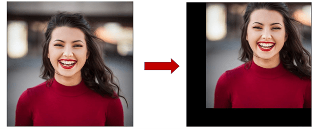
We have different types of simple Thresholding:

• THRESH_BINARY: If pixel intensity is greater than the set threshold, pixel value set to 255, else set to 0 .
• THRESH_BINARY_INV: Inverted or Opposite case of cv2.THRESH_BINARY.
• THRESH_TRUNC: If pixel intensity value is greater than threshold, it is truncated to the threshold. The pixel values are set to be the same as the threshold. All other values remain the same.
• THRESH_TOZERO: Pixel intensity is set to 0, for all the pixels intensity, less than the threshold value.
• THRESH_TOZERO_INV: Inverted or Opposite case of cv2.THRESH_TOZERO

FUNCTION USED   :  cv2.threshold()

It takes 4 arguments

• First argument      :  Source image (grayscale image)
• Second argument :  Threshold value
• Third argument     :  Maximum value to assign
• Fourth parameter : Types of simple Thresholding

The function returns two values. The first is the threshold that was used and the second output is the thresholded image.

Below is the implementation in python:-

Adaptive thresholding-

 In simple thresholding we used one global value as a threshold. But if an image has different lighting conditions in different areas. In that case, adaptive thresholding can help. This algorithm determines the threshold for a pixel based on a small region around it. So we get different thresholds for different regions of the same image which gives better results for images with varying illumination.

Function used :  cv2.adaptiveThreshold()

In addition to parameters involves in simple threshing except the thresholding value we have 3 more parameters here

1. Adaptive Method :  It decides how thresholding value is calculated.
   1. ADAPTIVE_THRESH_MEAN_C : threshold value is the mean of neighbourhood area.
   2. ADAPTIVE_THRESH_GAUSSIAN_C : threshold value is the weighted sum of neighbourhood values where weights are Gaussian window.
2. Block Size:  It decides the size of neighborhood area.
3. C : It is just a constant which is subtracted from mean or the weighted mean calculated.

Let’s see the implementation of it in Python-

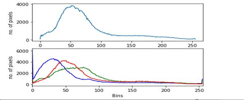
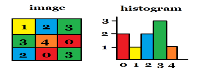
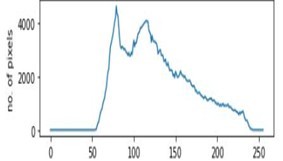
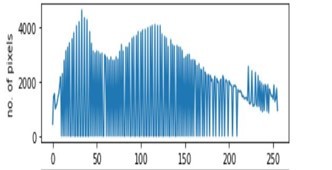
Histogram of an image-

Before we see the working of the ostu’s binarization we need to have knowledge of the histogram of an image. It is a representation of the distribution of the data. Histogram of an image represents the relative frequency of occurrence of various pixels in an image.

We use calcHist() function to find the histogram. Let’s familiarize with its parameters:

1. images : source image
2. Channels: It is the index of channel for which we calculate histogram. if input is grayscale image, its value is [0]. For color image, you can pass [0], [1] or [2] to calculate histogram of blue, green or red channel respectively.
3. Mask: To find histogram of full image, it is given as “None”. But if you want to find histogram of particular region of image, you have to create a mask image for that and give it as mask.
4. histSize : this represents our BIN count. Need to be given in square brackets. For full scale, we pass [256].
5. Ranges: this is our RANGE. Normally, it is [0,256].

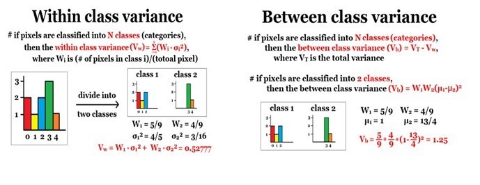
OTSU Binarization-

• In global thresholding, we used an arbitrary chosen value as a threshold. In contrast, ostu’s binarization automatically calculates a threshold value from image histogram.
• The threshold()function is used, where cv.THRESH_OTSU is passed as an extra flag. The threshold value can be chosen arbitrary. The algorithm then finds the optimal threshold value which is returned as the first output.
• The brief working of this algorithms can be understand using the below images, considered the histogram as shown below,

Suppose we choose the threshold value T=2, then the image is separated into two classes, which are Class 1 (pixel value<=2) and Class 2 (pixel value>2) as shown in below fig. We can say that these two classes represent the background and foreground of the input image respectively. (Class 2 can be the background if the foreground is darker than the background) , then we will calculate the within class variance and tries to minimize it, and calculate the between class variance and tries to maximize it, if for a chosen threshold we get the min. within class variance and max. between class variance then we will say that it will be our threshold.

Below is the implementation of the OTSU binarization

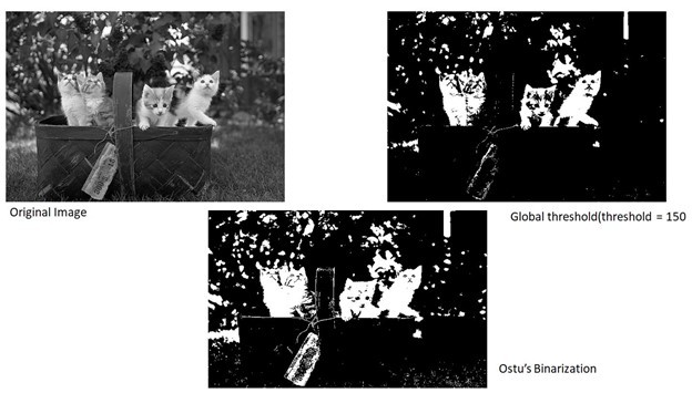
Image Enhancement in OpenCV :-

Image enhancement is one of the most important techniques in Opencv, it is one of the very basic task that we performed in our day to day life.

During the preprocessing of the images, few image can a high contrast or low brightness or extreme high brightness, in order to enhance them we have many techniques in openCV some of them are :

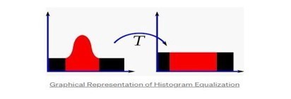
Histogram Equalization-

• • Histogram equalization helps us to normalize the brightness and the contrast in an image. It takes grayscale image as the input. This can also be called as global histogram equalization.
  • We will use equalizeHist() function in OpenCV for histogram equalization. Basically it normalizes the brightness and also increases the contrast.
  • To enhance the image’s contrast, it spreads out the most frequent pixel intensity values or stretches out the intensity range of the image as can be seen in below fig. By accomplishing this, histogram equalization allows the image’s areas with lower contrast to gain a higher contrast.

Below is the implementation of the histogram equalization-

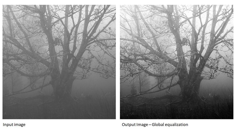
You can compare the above two images and their corresponding histograms.

CLAHE (Contrast Limited Adaptive Histogram Equalization)-

This is the adaptive histogram equalization, in this the image is divided into small blocks called “tiles” (tileSize is 8×8 deafult in opencv).  and then histogram equalization is applied,

If any histogram bin is above the specified contrast limit (by default 40 in OpenCV), those pixels are clipped and distributed uniformly to other bins before applying histogram equalization. In the end bilinear interpolation is applied to remove artifacts in tile border.

It gives better result than the global histogram equalization. It can be applied on grayscale as well as colour images.

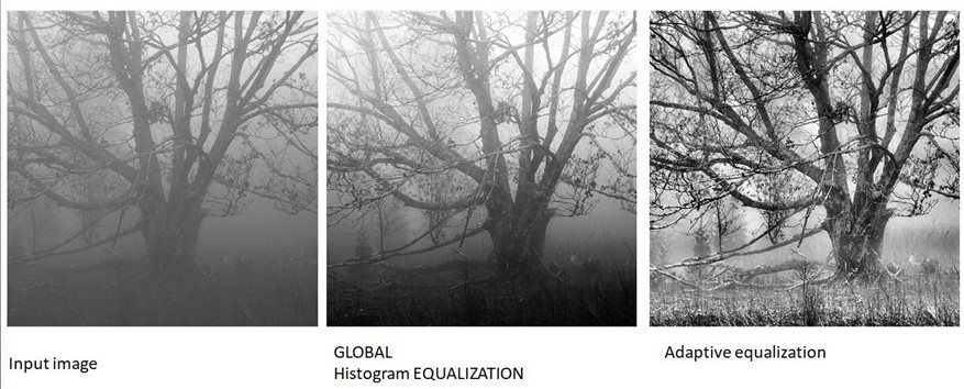
Here we can observe the result and can confidently see that the CLAHE performed much better as compare to the simple histogram equalization and it is expected.

So far, we have covered the basic function in OpenCV, along with the thresholding and image enhancement using OpenCV. This article is basically a kick start to your computer vision journey, so practice all those things and try to understand the working as well.

That’s all from my side, thanks for your time. We will be seeing you on the another article on OpenCV in which we will be covering some more useful functions in OpenCV

Related posts:

Face Detection using OpenCV Important Functions of OpenCV OpenCV Face Mask Detector using RetinaNet Model Introduction to GANs in Computer Vision