
Introduction:-
In the previous article on ‘OpenCV: Beginning for the Computer Vision enthusiast’, we have talked about the basic and the most useful function in the OpenCV that helps us to build the computer vision projects. So, in this article we are going to see some more important functions in an OpenCV that helps us in the preprocessing stage of the building the classifier. We will be seeing some ways to denoise the images, create contour on images, masking, and morphological operation.
Before moving forward, you need to have the basic knowledge of the OpenCV, if you are not aware of that then I highly recommend you to click here to check the above mentioned article.
Table of content-
- Blurring or smoothing of images in OpenCV
- Edge detection
- Contour detection
- Bitwise operation in OpenCV
- Morphological operation
Blurring or smoothing of image in OpenCV
We will start the formal definition of the blurring so ‘Image Blurring refers to making the image less clear or distinct’. It is done by convolving the image with low pass filter kernels. I hope you guys are aware of the How we convolve the image.
After reading the definition of the image blurring now the question arises what is the benefit of blurring an image?
Well, blurring helps us to remove the various unwanted noise in an image. So whenever we are working on the image dataset We come across various kinds of noises in image, these noises can affect the accuracy of the model, so in order to remove the noise, we often use the blurring methods which can significantly reduces the noise in image.
Advantages of Blurring-
- Blurring helps us to remove the amount of high frequency content (Noise) in an image; it is generally used before thresholding and edge detection.
- Blurring helps by reducing the detail in an image so that we can easily find objects that we are interested in.
- By blurring, Low intensity edges are removed.
- It helps in smoothing of the Images.
Now OpenCV has different Types of filter to blur the images. We will go through one by one on each type of blurring:-
Average Blurring:-
It is the simplest blurring technique; It simply takes the average of all the pixels under the kernel area and replaces the central element.
Below fig. shows the 2*2 Average kernel:
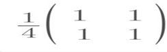
In OpenCV we have a single line function for performing the average blurring i.e. blur(source image, kernel dimension), we need to pass the source image, and the kernel dimension.
Let’s see the implementation in python-


Gaussian Blurring:-
Gaussian blurring is helpful to reduce the Gaussian noise in an image. It is highly effective filter to remove the Gaussian noise from the image as compare to other filters.
Gaussian blurring is generally used in a preprocessing stage in our deep learning models, Because whenever we perform resizing of an image, it often includes the Gaussian noise in an image.
We have the following openCV function for the gaussian blurring : GaussianBlur()
- We have four parameters in this function
- Input image
- Kernel size
- Standard deviation in x direction(sigmaX)
- Standard deviation in y direction(sigmaY)
Note : If zero is passed as standard deviation then it will calculated from the kernel size. Before moving to implementation let’s see how a gaussian noise looks like:
Let’s check out the Python implementation of it-


The amount of the blur can be increased with the increase in the kernel size.
So, now observing the results we can say that the Gaussian noise is not removed completely, but It has reduced to an significant amount, Now I want you guys to save the picture and check the result with all the other blurring techniques, well Gaussian blur will give you the best result.
Median Blurring :-
The Median Filter is a non-linear digital filtering technique often used to remove noise from an image or signal, whereas the average and the Gaussian are the linear filtering techniques.
Median blur takes the median of all the pixels under the kernel area and the central element is replaced with this median value. This blurring method is highly effective against salt-and-pepper noise in an image.
OpenCV function for median blurring : medianBlur()
- We have four parameters in this function
- source image
- Kernel size (if kernel is 5*5 then pass only 5)
Below is the implementation in python-

Here we can observe the effect of median filter and Gaussian filter on the salt and pepper noise, and can confidently say that the median filters works the best, it remove the complete salt and pepper noise from the image.
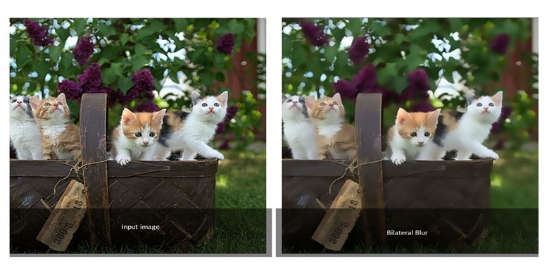
Bilateral Filtering:-
A bilateral filter is a non-linear, edge-preserving, and noise-reducing smoothing filter for images.
It replaces the intensity of each pixel with a weighted average of intensity values from nearby pixels. This weight can be based on a Gaussian distribution. Thus, sharp edges are preserved while discarding the weak ones.
OpenCV Function for bilateral blurring: bilateralFilter()
Parameters to pass in this function:-
- Input Image
- D (Diameter of each pixel neighborhood that is used during filtering)
- SigmaColor
- sigmaSpace
- borderType
The highlight of this filter is that it preserves the sharp edges in the image.
Let’s see the Python implementation-
We will see the effectiveness of bilateral filtering to preserve in the sharp edges in the next section.
Edge Detection:-
Edges are very useful features of an image that can be used for different applications like classification of objects in the image and localization. Deep learning models calculate edge features to extract information about the objects present in image.
In OpenCv we have a popular edge detection algorithms i.e. Canny edge detection algorithm, we will see the brief working of the Canny edge algorithm.
Canny Edge Detection is a popular edge detection algorithm available in opencv.
The main stages of this algorithms is :
- Noise Reduction – It uses the Gaussian filter to remove the noise in an image.
- Intensity Gradient of the image- The smoothen image is further processed through a sobel filter, to calculate the edge gradient for each pixel.
- Non-maximum Suppression- Non-max suppression is used to suppress the unwanted pixel which does not have contribution in the edges.
- Hysteresis Thresholding –This stage classifies edges and non-edges. The two thresholds passed are minVal and maxVal. Any edges with intensity gradient more than maxVal are considered as edges and those below minVal are not considered as edges. Those who lie between these two thresholds are classified edges or non-edges based on their connectivity. If they are connected to “sure-edge” pixels, they are considered to be part of edges otherwise not.
In OpenCV we have a single line function that’s helps us to implement the above algorithm i.e. Canny()
Parameters to pass in this function:-
- Input Image
- Minimum threshold (minVal)
- Max threshold ( maxVal)
Note : The higher the thresholds, the cleaner the edges.
Let’s see the python implementation:-

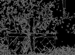
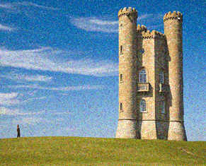
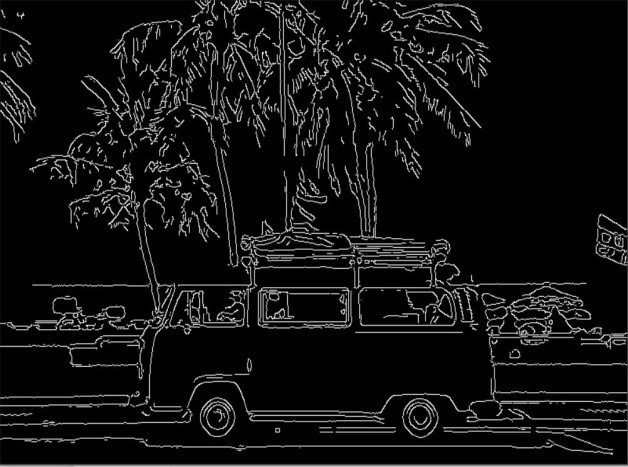
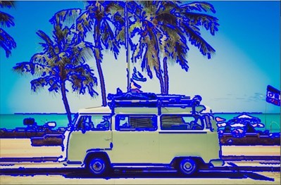
Image:- Source Image

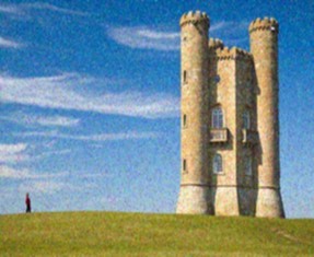
We can check the result of the canny edge detection algorithm, here we can see that even after applying high threshold values there is a lot of background noise, in order to reduce it we can use the bilateral filter before canny which will helps us to remove the weak edges that are in the background and preserve the sharp edges as discussed in the previous section;
Let’s check the results-
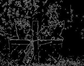
We can observe the result and confidently say that bilateral filtering work well for removing the weak edges. We can also use variety of the filter in order to improve the edge detection in image.
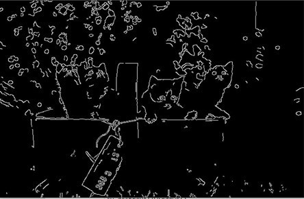
Contour detection:-
The contours are a useful tool for shape analysis and object detection and recognition, Contours is simply a curve joining all the continuous points (along the boundary), having same color or intensity.
In OpenCV contour detection is applied after the canny edge filter.
Function used :
- findContours() – Used for finding the contours, the function return contours and hierarchy
- Paramters
- Input image
- contour retrieval mode
- contour approximation mode
- Paramters
- drawContours() –To plot the contours
- Parameters
- source image
- contours which should be passed as a Python list
- index of contours (useful when drawing individual contour. To draw all contours, pass -1)
- color, thickness etc.
- Parameters
- findContours() – Used for finding the contours, the function return contours and hierarchy
Let’s check the Python implementation-

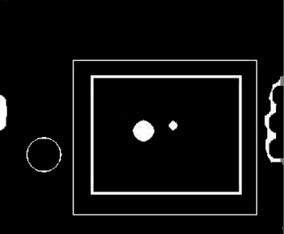
Bitwise operation:-
We can also perform the bitwise operation with images, bitwise operation include AND, OR, NOT and XOR. These are very useful in masking of the image so that we can extract the region of the interest in image.
Let’s see how we can perform the bitwise operation with images:


Image:- OR


Morphological Operation:-
A collection of non-linear operations related to the shape or morphology of features in an image is known as Morphological Operation in Image Processing.
It is normally performed on binary images.
We have many types of morphological operation which are
1. Erosion
The basic intuition about the erosion is that it erodes away the boundaries of the foreground objects. The kernel slides through the image. A pixel in the original image (either 1 or 0) will be considered 1 only if all the pixels under the kernel are 1, otherwise it is eroded (made to zero).
We have few advantages of erosion:
- This reduces the thickness of white region in an image.
- Erosion can be useful for removing small white noises.
Function used: cv2.erode()
Parameters passed in this function-
- Source image
- Kernel
- of iteration
2. Dilation-
It is just opposite of erosion. Here, a pixel element is ‘1’ if at least one pixel under the kernel is ‘1’.
It increases the white region or the foreground object in the image. It is also useful in joining broken parts of an object.
Function used: cv.dilate()
Parameters passed in this function-
- Source image
- Kernel
- of iteration
3. Opening-
Opening is just another name of erosion followed by dilation. Normally, in cases like noise removal, erosion is followed by dilation. Because erosion removes white noises but it also shrinks our object. So we dilate it. Since noise is gone, they won’t come back, but our object area increases.
Function used: cv.morphologyEx()
Parameters passed in this function-
- Source image
- MORPH_OPEN
- Kernel
4. Closing-
Closing is reverse of Opening, Dilation followed by Erosion. It is useful in closing small holes inside the foreground objects, or small black points on the object.
Function used: cv.morphologyEx()
- Parameters
- Source image
- MORPH_CLOSE
- Kernel
5. Morphological Gradient
It is the difference between dilation and erosion of an image. The result will look like the outline of the object.
Function used : cv.morphologyEx(img, cv.MORPH_GRADIENT, kernel)
Let’s check the implementation of all the above morphological operation-


Let’s look at the use case of the morphological operation –
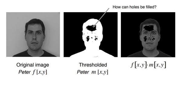
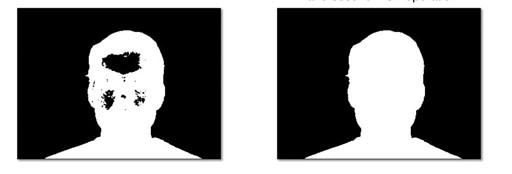
Now as the hole is now filled, we can apply the AND operation between the final thresholded image and the original image to segment out the face.
So this is all about the morphological operation.
End Notes-
In the series of the of two articles I have covered the most important functions of OpenCV that will help you in your computer vision journey, Now I will suggest you to implement those function by yourself, because that’s the only way for you to understand the things better.
The things I have covered will help you in every deep learning model that will require image processing. Discussed functions can also be used in building the good real time project like FACE DETECTION, AI FINGER COUNTING, Road Lane detection, Ai virtual Mouse and many more things, so make some great project And try to implement this learning while creating your own computer vision project.
That’s all from my side, Have a great learning ahead. If you like the article then don’t forget to leave claps on article. It motivates us to write more such awesome Data Science content. 🙂


