
Introduction-
Convolutional Neural networks also known as ConvNets or CNN. ConvNet is famous for image analysis and classification tasks and so are frequently used in machine learning applications targeted at medical images. They also have an excellent capacity in sequent data analysis such as NLP(Natural Language Processing).
Some of the application of CNN that might excite you –
Example 1. Image with and without background blur


Example 2. Background Subtraction
Portrait mode on iPhone X


Example 3. Google Photos


Example 4. Autonomous Driving Cars
Compared to other classification algorithms, CNN requires much less preprocessing and can give better performance with increase in training data.
CNN is made up of one input layer, multiple hidden layers, and an output layer in which hidden layers structurally include convolutional layers, ReLU layers, pooling layers, fully connected layers, and normalization layers. So, ConvNet has two main operations, namely convolution and pooling.
Convolution operation with input data using multiple filters is able to extract feature maps from the data set, through which their important spatial information can be preserved.
Pooling operation is also known as subsampling operation. It is used to reduce the dimensionality of feature maps from the convolution operation. Most common types of pooling are Max pooling and average used in CNN.
Here comes the big advantage of reducing the count of weights required to be trained. Unlike the standard neural network, each neuron in the layers is not connected to all of the nodes (neurons) in the previous layer but is just connected to nodes in a special region known as the local receptive field.
Convolution layer-
Given Input sample(image) is convolved with numerous filters.Each of the kernel results in a distinct feature map.
First things is to overlay the filter on to the input, perform element wise multiplication, and add the result.

Move the filter right by one position (stride=1), and do the same calculation and get the next result. And this continues for the whole input

Want to see what’s convolution capable of ???

Let’s consider below 2 filters –
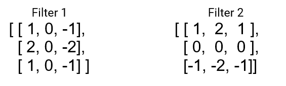
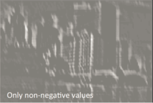
The result of convolution with Filter 1-

Isn’t it cool, we can find vertical edges in the image now..
The result of convolution with Filter 2-

Now we obtained the horizontal lines.
So, now we can see how doing convolution with different filters can make sense to obtain different features of an image and together make some conclusions and results out of it. Lets go through some more basic parameters for this convolution operation.
Stride-
It is the number of pixels shift over the input matrix. When the stride is 2 then the filters move 2 pixels at a time and so on

Padding–
We know that after convolution the size of image shrinks, and if it passes through numerous count of filters it will lose its information and performance will degrade, which can be a problem in deeper networks. In this scenario padding can play a vital role in preventing this vanishing problem. It allows us to use a CONV layer without necessarily shrinking the height and width of the volumes.
It is also observed that information at the border of an image is wasted. Without padding, very few values at the next layer would be affected by pixels as the edges of an image.

Important terminologies:-
“valid” padding- means no padding, images size reduces after convolution.
“same” padding-means padding is done so that the output dimension is the same as the input.
ReLU activation layer –
The rectifier serves to break up the linearity, that we might impose on an image when we put it through the convolution operation. They speed up the training process by preventing the vanishing gradient problem. All operations seen so far: convolutions, elementwise matrix multiplication and summation are linear.

If we don’t have a non linearity, we will end up with a linear model that will fail in the classification task.
In below images, you can see the output of different operations-


Note: Other non linear functions such as tanh or sigmoid can also be used instead of ReLU, but ReLU has been found to perform better in most situations.
Pooling Layer-
This layer simplifies the information and reduces the scale of feature maps. It is commonly used immediately after the convolutional layer. Pooling layer makes a condensed feature map from each feature map in a convolutional layer. This layer is also called the subsampling layer. Pooling operation can be performed in various types such as geometric average, harmonic average, maximum pooling
Maximum pooling Vs Average pooling:-
Max-pooling and average-pooling are the most used types of pooling. The pooling layer is necessary to reduce the computational time and overfitting issues in the CNN.

Which is best Pooling Method??
We cannot say that a particular pooling method is better over other generally. The choice of pooling operation is made based on the data at hand. Average pooling – smooths out the image , the sharp features may not be identified. Max pooling – selects the brighter pixels from the image, useful when the background of the image is dark and we are interested in only the lighter pixels of the image.
For example: in MNIST dataset, white color digits with black background. So, max pooling is used.


Fully connected layers –
These are final layers in the CNN structure that can be one or more layers and placed after a sequence of convolution and pooling layers. It comprises the composite and aggregates of the most important information from all procedures of CNN. These layers will be providing a feature vector of the input data, which is used for classification or prediction.
The last layer of fully connected layers is the softmax layer, it determines the probability of input image belonging to each target class .
Calculation of output dimension –
CNN Output Size Formula :-
The output size O is given by this formula:- O=[(W-K+2P)/S] +1
Where-
- W- Input Size
- K-Kernel Size
- P-Padding Size
- S-Stride
Note: Stride by default is 1 ,if not provided.
For Example- Let’s say, we’ve a convolutional layer with an input image with (128*128*3) size with 40 filters then output dimension of feature map would be-
O=[(128-5+0)1]+1 = 124
So feature dimension would be (124*124*40)
This value will be the height and width of the output. However, if the input or the filter isn’t a square, this formula needs to be applied twice, once for the width and once for the height.
- Suppose we have an Nh×Nw input.
- Suppose we have an Fh×Fw filter.
- Suppose we have a padding of P and a stride of S.
The height of the output size Oh is given by this formula:-
Oh=(Nh-Fh+2P)/S +1
The width of the output size Ow is given by this formula:-
Ow=(Nw-Fw+2P)/S +1
Counting the number of parameters in Convolutional Layer-
Just multiply the shape of width M, height N, previous layer’s filters D and account for all such filters k in the current layer, and don’t forget the bias term for each of the filter.
So, number of parameters in a CONV layer would be : ((M * N * D)+1)* K).
Note:- Added 1 because of the bias term for each filter.
(( width of the filter * height of the filter * number of filters in the previous layer+1)* number of filters in current layer).
- Where the term “filter” refer to the number of filters in the current layer.
Approaching to application-
To design a ConvNet structure is a challenge because you will need to tune many hyperparameters carefully because they will have significant influence on the performance of CNN structure such as depth (count of convolutional, pooling, and fully-connected layers layers), number of filters, stride, pooling types and the number of units in fully-connected layers. Finding the proper hyperparameters combination needs experience and is often performed as a trial and error process.
There are two methods for applying CNN models that include: training from scratch and performing transfer learning by use of pre-trained models.
Method 1 – From scratch
You will have to define the number of layers and filters and will require massive amounts of data if the network is deep which is time-consuming because it’s challenging to get the correct labeled data. It will also have high computational cost.
Bigger challenge is there are many hyperparameters such as depth ,the number of filters, stride, pooling type and sizes, the number of units in fully-connected layers and it will be requiring experience to tune them correctly.
Method 2- Transfer learning
Pre-trained CNN models trained on similar kinds of tasks or data can be used without need of training again. This means that in transfer learning, the ability of pre-trained models to learn the complex function helps to train the new targets instead of training from scratch, you can freeze the pretrained layers and add some layers as per wish.
Transfer learning is a faster and easier method for applying deep learning, and it is not necessary to understand the structure and combinations of network layers.
Pre-trained CNNs available on tensorflow hub are freely downloadable and are trained on a huge number of the images with the aim of detection and classification (images) in a large number of classes (can be 1000). AlexNet, GoogleNe, SqueezeNet , ResNet , DenseNet-201 , Inception-v3 , and VGG are some of the famous pre-trained models used in transfer learning technique.
Article Credit:-
Name:- Ankush Deshmukj
Qualification-:- Linkedin


