
Introduction:-
In this article, we’ll talk about why Vector Space Models became popular in NLP realm. Then we’ll take deep dive into Word2vec Model.
As we all know that Machine learning models take vectors or arrays of numbers as input. When we work on the text data, we can not give words directly to the machine learning model. The first thing we must do is come up with a strategy to convert strings to numbers before feeding it to the model. This is also known as the “vectorization” of the text.
1. One hot encoding-
One hot encoding is the easiest idea to encode each word in your vocabulary. Consider the sentence “The cat sat on the mat”. (cat, mat, on, sat, the) are the unique words that present in this sentence. To represent each word, we have to create a zero vector with a length equal to the vocabulary, then place a one in the index that corresponds to the word. This approach is shown in the following diagram.
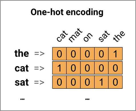
This approach is not efficient. A one-hot encoded vector is sparse (meaning, most indices are zero). Imagine we have 10,000 words in the vocabulary. To one-hot encode each word, we would create a vector where 99.99% of the elements are zero.
2. Encode word with a unique number-
In this approach we might try is to encode each word using a unique number. Consider the above sentence, we could assign 1 to “cat”, 2 to “mat”, and so on. We could then encode the sentence “The cat sat on the mat” as a vector like [5, 1, 4, 3, 5, 2]. This approach is efficient. Instead of a sparse vector, we now have a dense one vector (where all elements are full).
There are two drawbacks to this approach.
- Integer encoding is arbitrary. It does not capture any relationship between words.
- It can be challenging for a model to interpret. Because there is no relationship between the similarity of any two words and the similarity of their encodings, this feature-weight combination is not meaningful.
3. Word Embedding-
It gives us a way to use an efficient, dense representation in which similar words have a similar encoding. Importantly, we do not have to specify this encoding by hand. An embedding is a dense vector of floating-point values. The length of the vector is a parameter that we have to specify. Instead of specifying the values for the embedding manually, they are trainable parameters (weights learned by the model during training, in the same way, a model learns weights for a dense layer). A higher dimensional embedding can capture fine-grained relationships between words but takes more data to learn.
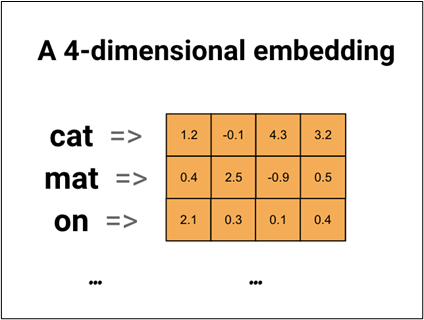
The above diagram shows word embedding for the sentence “The cat sat on the mat”. Each word is represented as a 4-dimensional vector of floating-point values.
Word2Vec Model:-
It is a family of model architectures and optimizations that can be used to learn word embeddings from large datasets. Tomas Mikolov et.al. from Google developed the Word2Vec algorithm.
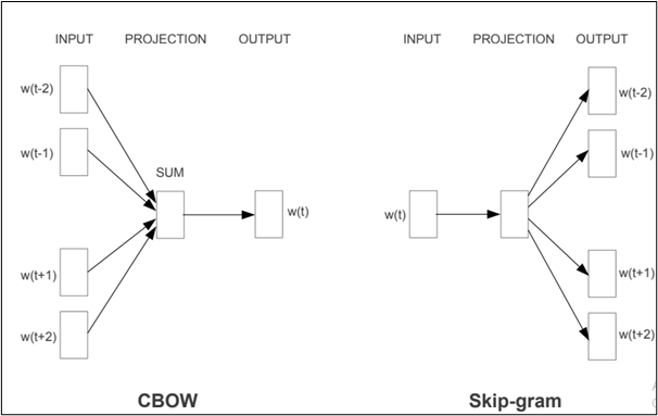
Continuous Bag of Words Model and Skip-grams model are two models were proposed in these papers-
- Skip-gram Model: It predicts context words (position independent) given centre word.
- Continuous Bag-of-Words Model: It predicts the middle word based on surrounding context words. The context consists of a few words before and after the current (middle) word. This architecture is called a bag-of-words model as the order of words in the context is not important.
Skip-Gram Model-
The model is trained on skip-grams, which are n-grams that allow tokens to be skipped. The context of a word can be represented through a set of skip-gram pairs of (target_word, context_word) where context_word appears in the neighbouring context of target_word. This model uses each current word as an input to a log-linear classifier with a continuous projection layer, and predict words within a certain range before and after the current word.
Consider the following sentence- The quick brown fox jumps over the lazy dog
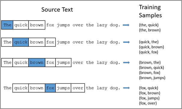
Fig 4: Training samples with window size = 2. Source
The context words for each of the 9 words of this sentence are defined by the window size. The window size determines the span of words on either side of a target_word that can be considered a context word.
In the above example, we have considered a window size of 2. On the right side, we have the training samples for target words such as The, quick, brown, fox.
Model Details-
The input vector will be a one-hot representation of a word with a dimension as 1xV, where V is the number of words in the vocabulary. The single hidden layer will have dimension VxE, where E is the size of the word embedding and is a hyper-parameter.
The output from the hidden layer would be of the dimension 1xE, which we will feed into a softmax layer. The dimensions of the output layer will be 1xV, where each value in the vector will be the probability score of the target word at that position.
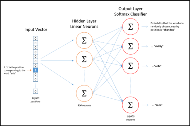
Fig 5: Architecture for the skip-gram model. Source
The training objective of the skip-gram model is to maximize the probability of predicting context words given the target word. For a sequence of words w1, w2, … wT, the objective can be written as the average log probability
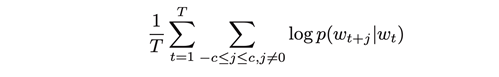
where c is the size of the training context. The basic skip-gram formulation defines this probability using the softmax function.
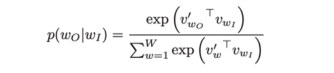
Where- v and v’ are target and context vector representations of words and W is vocabulary size.
Continuous Bag-Of-Words Model-
The task in CBOW is somewhat similar to Skip-gram, in the sense that we still take a pair of words and teach the model that they co-occur but instead of adding the errors, we add the input words for the same target word.
The dimension of our hidden layer and output layer will remain the same. Only the dimension of our input layer and the calculation of hidden layer activations will change, if we have 4 context words for a single target word, we will have 4 1xV input vectors. Each will be multiplied with the VxE hidden layer returning 1xE vectors. All 4 1xE vectors will be averaged element-wise to obtain the final activation which then will be fed into the softmax layer.
Problem with CBOW/Skip-gram-
The first thing is for each training sample, only the weights corresponding to the target word might get a significant update. While training a neural network model, in each back-propagation pass we try to update all the weights in the hidden layer. The weight corresponding to non-target words would receive a marginal or no change at all, i.e. in each pass we only make very sparse updates.
Secondly, for every training sample, the calculation of the final probabilities using the softmax is quite an expensive operation as it involves a summation of scores over all the words in our vocabulary for normalizing.
So for each training sample, we are performing an expensive operation to calculate the probability for words whose weight might not even be updated or be updated so marginally that it is not worth the extra overhead.
To overcome these two problems, The authors of Word2Vec addressed these issues in their second paper with the following two innovations:
- Subsampling frequent words to decrease the number of training examples.
- Modifying the optimization objective with a technique they called “Negative Sampling”, which causes each training sample to update only a small percentage of the model’s weights.
It’s worth noting that subsampling frequent words and applying Negative Sampling not only reduced the compute burden of the training process, but also improved the quality of their resulting word vectors as well.
Negative Sampling-
Negative sampling allows us to only modify a small percentage of the weights, rather than all of them for each training sample. We do this by slightly modifying our problem. To augment our formulation of the problem to incorporate Negative Sampling, all we need to do is update the:
- objective function
- gradients
- update rules
Instead of trying to predict the probability of being a nearby word for all the words in the vocabulary, we try to predict the probability that our training sample words are neighbors or not. So instead of having one giant softmax — classifying among 10,000 classes, we have now turned it into a 10,000 binary classification problem.
Consider the above example, when training the network on the word pair (“fox”, “quick”). The “label” or “correct output” of the network is a one-hot vector. That is, for the output neuron corresponding to “quick” to output a 1, and for all of the other thousands of output neurons to output a 0.
With negative sampling, we are instead going to randomly select just a small number of “negative” words let’s say 5 to update the weights for. (In this context, a “negative” word is one for which we want the network to output a 0). We will also still update the weights for our “positive” word (which is the word “quick” in our current example).
For our training sample (“fox”, “quick”), we can take five negative samples, say (“fox”, “juice”), (“fox”, “dinner”), (“fox”, “dog”), (“fox”, “chair”), (“fox”, “table”). For this particular iteration, we will only calculate the probabilities for quick, juice, dinner, dog, chair, table. Hence, the loss will only be propagated back for them and therefore only the weights corresponding to them will be updated.
The modified objective function is given by-
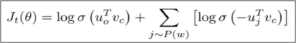
Here – sigmoid = 1/(1+exp(x)),
t is the time step and theta are the various variables at that time step, all the U and V vectors.
The first term tries to maximize the probability of occurrence for actual words that lie in the context window, i.e. they co-occur. While the second term tries to iterate over some random words j that don’t lie in the window and minimize their probability of co-occurrence.
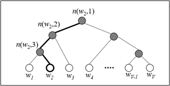
Hierarchical Softmax Classification-
The main motivation behind this method is to reduce the computational complexity from O(n) to O(log2 n). We do it with the usage of the binary tree, where leaves represent probabilities of words, more specifically, leave with the index j is the jth word probability and has position j in the output softmax vector.
Each of the words can be reached by a path from the root through the inner nodes, which represent probability mass along that way. Those values are produced by the usage of simple sigmoid function as long as the path we’re calculating is simply the product of those probability mass functions.
Let’s see what happens to the computation complexity if we divide our vocabulary into two equal non-overlapping groups, and change the classification process to first selecting the group.
P(group=i|x)=softmax(x∗Wgroupselect+bgroupselect)
References:-
- https://www.tensorflow.org/tutorials/text/word_embeddings
- https://www.tensorflow.org/tutorials/text/word2vec
- https://cs224d.stanford.edu/lecture_notes/notes1.pdf
- https://towardsdatascience.com/nlp-101-word2vec-skip-gram-and-cbow-93512ee24314
- https://towardsdatascience.com/nlp-101-negative-sampling-and-glove-936c88f3bc68
Article Credit:-
Name: Sameer Koleshwar
Qualification: M.Tech in Signal Processing and Machine Learning, NITK
Research Area: Natural Language Processing Linkedin


